A quite complete article about how to control opponent’s score in some games, using a nice part of mathematics called Game Theory.

This article is derived from this paper from mathematicians Press & Dyson. The original work isn’t very understandable for everyone, so I decided to work on it and publish it with illustrations and graphs so everybody can understand!

For maths lovers: see you in part 5.

After reading this article, you may want to try your own strategies with these ressources I made just for you!

1. Prisoner’s dilemma

The story

You stole the bank with your partner in crime. You just had the time to hide the money when the sirens sound. You see the police coming and you run. Too late: the police is here! You fight with a policeman while trying to escape, but they manage to arrest you anyway. You are now at the police station. But they do not have any evidence that you two are the thieves!

A clever policeman takes you aside and says

Here’s the deal: you will decide the fate of your friend. You have two choices.

• If you lie and say he is innocent, we will sue you for fighting with the police. You’ll get 1 year in prison.
• If you betray him, you’re immediately free! However he’ll get the maximal sentence: in jail for 10 years.

Of course, it’s the same deal for your partner… If you betray each other, you’ll share your sentence and go 5 years each in prison.

The prisoner thinks a few minute.

My fate will depend on his choice, so :

• If my friend betrays me, I better have to betray him too: I’ll go to prison 5 years instead of 10.
• If he lies and protect me, I should betray too : I’ll never go to prison, instead of wasting my life during 1 year…

In any case, it’s better to betray. If he thinks the same, I have no reason to cooperate.

At the end, they both betray each other and go to prison 5 years, whereas they could have cooperated and go to prison only 1 year…

That is the prisoner’s dilemma.

Representing games

The prisoner’s dilemma is one of the fundamentals of Game Theory.

As every game in “normal form”, it’s described by 3 things (see more):

• Players
• Strategies for each player. It can be anything: {heads, tails} or {bet 1€, bet 5€, bet 10€}
• Utility function: it maps every situation (strategies of every player) to a gain (or a loss)

A 2-players game with finite strategies is often represented as a mere table. So it sums up like this for example:

X Y	Ace	Queen
King	(-1, 1)	(1, -1)
10	(-3, 3)	(-1, 1)
9	(-6, 4)	(-2, 5)

In this game, if X plays a 10 and Y plays the Ace, Y will get 3 points and X will lose 3 points. The mean value of utility for X is -2, his cards aren’t good!

In Game Theory, the utility (the gain function) can be anything too. It can be expressed in euros, happiness, pastries, or a mix of all three!

What about the prisoner’s dilemma?

It’s a 2 players (X and Y) game with 2 strategies each: Cooperate (C) or Defect (D).

X Y	Cooperate	Defect
Cooperate	(3, 3)	(0, 5)
Defect	(5, 0)	(1, 1)

Here we took the opposite situation described in the little story. It looks more like a loot sharing situation.

The numbers (0, 1, 3, 5) can change, but it is a classical example.

Equilibria

The main goal of Game Theory in to find equilibria: these are special situations that allows one to guess what to do.

One of the most well-known is the Nash Equilibrium: it is a situation where no player can strictly benefit from deviating to another strategy, knowing that the others play according to the given situation. For the prisoner’s dilemma, it’s the strategy {D, D} (that lead to a utility of 1 to everyone) : as exposed in the story, a player which is rational have no reason to change its strategy and cooperate, as it leads to a smaller utility!

Another Equilibrium is the Pareto Optimum. It is a situation where you can’t increase the utility of a player (by changing its strategy) without reducing the utility of another player. The strategies {C, C}, {C, D} and {D, C} are Pareto Optimums. For example, from {C, C} to increase the utility of player X, he can only do that by reducing the utility of Y.

The paradox

The ‘paradox’ can be summarized in one sentence:

In the Prisoner’s Dilemma game, none of Nash Equilibria are Pareto Optimums.

The only Nash Equilibrium is the situation {D, D}. And it isn’t a Pareto Optimum: if both players cooperate, they can simultaneously increase their gain! But since it is a Nash equilibrium, neither player has any interest in doing that. Playing both Cooperate is sub-optimal as a player could easily betray to increase his winnings!

The strategy Cooperate is said “dominated” by the strategy “Defect”, because whatever the opponent do, it is always better to betray.

The situation {C, C} is called the “social optimum”, as it is the highest total utility. But it will never be played.

But what if the two players can talk to each other? There might be betrayals, it’s just talk.

So what if they can’t, but they can play repeatedly?

Will it build trust or resentment?

2. Iterated Prisoner’s dilemma

New behaviors

If one knows what the opponent have played during the last 50 rounds, it is more likely to know what to chose.

But it would induce very complicated algorithm to find the right strategy.

In fact, the mathematicians Press and Dyson have found that for infinite rounds (and it will work for an enough big number of rounds in practice) of the same game, it is enough to know the action of the previous round to make a good strategy.

So we will adapt our strategies to the actions of the previous round!

New strategies

Pure strategies

If we both cooperated, let’s cooperate again. If I cooperated but the opponent betrayed me, let’s betray him next round. If we betrayed him and he attempted to cooperate, let’s betray him again, it works! If we both betray, we’ll try to both increase our gain by cooperating.

We just build the following strategy:

X Y	C	D
C	Cooperate	Defect
D	Defect	Cooperate

We will simplify it as this:

X Y	C	D
C	1	0
D	0	1

With 1 meaning 100% chance for X to cooperate the next round and 0 meaning 0% for X chance to cooperate the next round (100% chance of betrayal).

We can have other strategies:

The naive

X Y	C	D
C	1	1
D	1	1

The thief

X Y	C	D
C	0	0
D	0	0

The copycat a.k.a tit-for-tat (copies what the opponent played last turn)

X Y	C	D
C	1	0
D	1	0

A lot of strategies exist!

Mixed strategies

You can even randomize the chances to cooperate.

The undecided (0.5 meaning 50% chance to cooperate)

X Y	C	D
C	0.5	0.5
D	0.5	0.5

The cautious

X Y	C	D
C	0.99	0.5
D	0.9	0.1

You can invent your own!

We just need one thing more before comparing strategies: the initial situation! It doesn’t depend on the “last round” because it’s the first…

Let’s fight!

One vs one

We will compare two strategies:

The resentful: betray him once, he will always betray! He cooperates first.

X Y	C	D
C	1	0
D	0	0

The cautious. He cooperates first.

X Y	C	D
C	0.99	0.5
D	0.9	0.1

Here’s what happened when playing 2,000 rounds (blue for the cautious and red for the resentful)

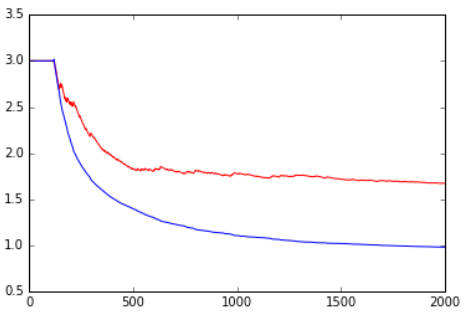
The mean gain was 3 while they both cooperate, and then it breaks down when the cautious betrays for the first time (he had 1% chance to betray in the {C, C} situation). Then, the resentful always betrayed, even when the cautious tried to cooperate. That’s why the gain of the cautious went down to 1 (as the Nash Equilibrium {D, D} utility is 1). Sometimes the cautious attempt to cooperates and gets 0 while the resentful gets 5 by defecting.

There are even more graphs than strategies, so try it out with my script just here!

One vs all

Comparing 2 strategies at a time isn’t very efficient. I entered all strategies in a database so I can choose a strategy and it displays the result for a given number of rounds against all the strategies (including itself).

Everything is here again. Just create your own strategy and launch the script, everything will be computed automatically ;)

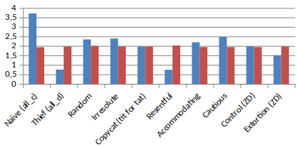
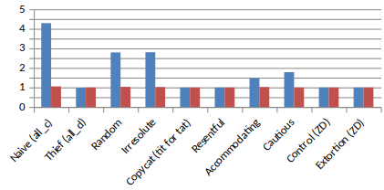
For example, we can see the results for the strategy

The irresolute

X Y	C	D
C	0	0
D	1	1

against some other strategies, for 10,000 rounds.

It wins against some but loses against some…

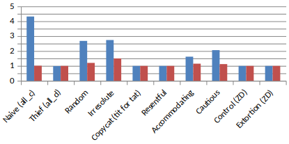
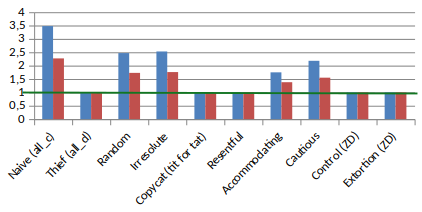
All vs. all

The mean score for a given strategies against all the other strategies doesn’t mean anything because it relies on the number of other strategies (and this shouldn’t matter).

A good thing that can be done is just counting the beaten strategies.

We can easily see that the thief wins every time, as it always play the dominent strategy.

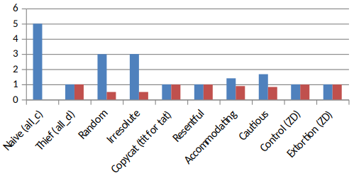
But it isn’t the strategy with the highest mean score: tit-for-tat have a much better score for example.

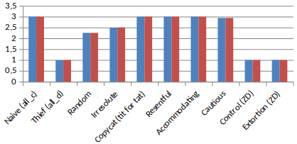
It is interesting to see that following this strategy will cause you to have the same score than the opponent at the end of the 10,000 rounds.

Conclusion

There are no perfect strategies here. Maybe we have to find better ones, that allow to win with a high score while defeating the other!

I told you in the title that we can do better: control the opponent’s gain.

3. Optimized Strategies

Control

If you choose the right strategy, you can set the mean opponent’s score to any value between 1 (the utility for the Nash equilibrium) and 5 (the maximal gain).

For example with Control 2, we set the opponent’s score to 2!

X Y	C	D
C	0.9	0.7
D	0.2	0.1

Why 0.9, 0.7, 0.2 and 0.1? How do we chose the right coefficients? The answer is quite complicated but you can find in in part 5.

Notice that the opponent’s score is always 2 in this graph. But we might have a score lower than 2, so this strategy is quite useless, even if it it interesting…

You can even set the opponent’s score to 1, the minimum possible! (as it is the utility at the Nash equilibrium)

Control 1

X Y	C	D
C	0.0	0.0
D	0.5	0.0

We can see some defects… in fact, the more you tend to 1, the more time it takes, and it seems 10,000 rounds isn’t enough for some strategies to go to its limit.

Moreover, our score in incredibly low, even lower than for Control-2.

What’s incredible is that you can’t control your own score by doing this. You will never be able to do that in Game Theory, because it is not interesting. It in not a strategy, but full control, and thus uninteresting.

This strategy is interesting, but not satisfying enough.

We don’t want to control the opponent’s score, we want to have better than him every time.

Extorsion

Even if we can’t control our own gain, it still is possible to control the ratio of our score to the opponent’s.

Extorsion 2 set our score two times higher than the opponent’s!

X Y	C	D
C	8/9	0.5
D	1/3	0.0

In fact, it is not really the score which is twice higher, but rather the part above 1 (the Nash Equilibrium)

If we are greedy, we can try to set the ratio to 100. But here’s what happen:

In fact, 100x0 = 0. By trying to reduce the opponent’s score to 0 (in fact, 1 as we saw), we are reducing our own score.

Extorsion vs. control

We can make these two incredible strategies fight each other.

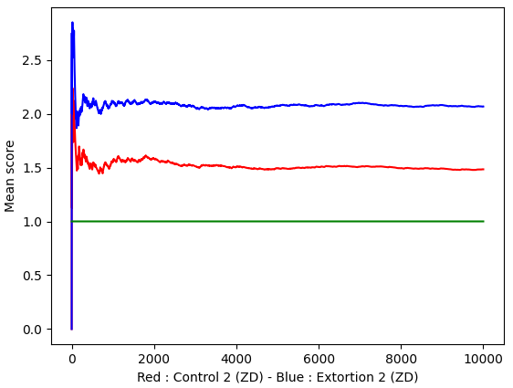
They are compatible! Control-2 set the Extorsion’s score to 2 and Extorsion-2 makes sure that his score is twice the Control’s score (relatively to the utility at Nash Equilibrium of course).

The winning strategy!

The Extorsion strategy will always have a better score than any of its opponents, or at least the same than them. To maximize the score, don’t be too greedy at apply a factor 2 or 3 (remember that 100x0 = 0).

Learn how to compute it in part 5 or use my algorithm to experiment it without maths.

4. Real life application

Wow. If you have read this far, you must wonder:

What is it useful for? These strategies were nice, but I’ll never play 10,000 prisoner’s dilemma?

There are many games that can look as Prisoner’s dilemma. Here’s a short list:

• economic competition
• patent owning
• animal cooperation (bats for example must learn to cooperate sometimes and betray other times)
• couple life (each decision can be a dilemma according to your preferences, even if it is not always a big deal)

Remember that if you want to maximize your happiness, do not betray every time. But do not cooperate each time: think about yourself!

Randomizing you gives you a better mean utility.

Think about this!

5. Appendix: Real maths. Proofs.

Game in normal form

A game is represented by 3 elements:

$$\mathcal{G}=\{\mathcal{N}, S, \mu\}$$

• a set of players $\mathcal{N}= {P_{1}, P_{2}, P_{3}, …, P_{N}}$
• a set $S={S_{1}, S_{2}, S_{3},…, S_{N}}$
  • the set $S_{i}$ is the set of strategies for player $P_{i}$
  • $S_{i}$ can be anything: {heads, tails} or {bet 1$, bet 5$, bet 10$}
  • we call $\mathfrak{S} = \times_{i=1}^{N}S_{i}$ the set of every situation possible
• a utility function: $\mu:s \in \mathfrak{S} \mapsto (g_{1}, …, g_{N}) \in \mathbb{R}^N$

A zero-sum game is such that

$$\forall s \in \mathfrak{S}, \sum_{i=1}^{N} \mu_{i}(s) = 0$$

A symmetrical two-players game is such that

$$\forall (s_{1}, s_{2}) \in \mathfrak{S}, \mu_{1}(s_{1}, s_{2})=\mu_{2}(s_{2}, s_{1})$$

Prisoner’s dilemma generalized

We often represent two-players game with a matrix. The prisoner’s dilemma is a symmetrical game with the following coefficients and constraints:

X Y	C	D
C	(b, b)	(d, a)
D	(a, d)	(c, c)

With $a > b > c > d \geq 0$

In fact $\mu(C,D)=(d, a)$ and so on.

Strategies: general form

The general form for a 1-memory strategy is a vector $p = (p_{1}, p_{2}, p_{3}, p_{4}) \in [0, 1]^4$ such as

X Y	C	D
C	$p_{1}$	$p_{2}$
D	$p_{3}$	$p_{4}$

Press and Dyson’s work

Relation between the scores

A step from a round n to another (n+1) might be represented with a Markov transition matrix.

$$ M(p, q) = \begin{pmatrix} p_1 q_1 & p_1 (1-q_1) & (1-p_1) q_1 & (1-p_1) (1-q_1) \\\ p_2 q_3 & p_2 (1-q_3) & (1-p_2) q_3 & (1-p_2) (1-q_3) \\\ p_3 q_2 & p_3 (1-q_2) & (1-p_3) q_2 & (1-p_3) (1-q_2) \\\ p_4 q_4 & p_4 (1-q_4) & (1-p_4) q_4 & (1-p_4) (1-q_4) \\\ \end{pmatrix} $$

We can easily verify

$$ \forall (i,j), 0\le a_{ij} \le 1 $$

$$ \forall i, \sum_{j}M_{ij}=1 $$

The Markov matrix has 1 as eigenvalue as every Markov matrix.

1. Let M’=M-I. M’ have 0 as eigenvalue so $det(M’)I=0$
2. According to the adjoint matrix formula, $adj(M’)M’=det(M’)I=0$
3. Let’s call u one of the eigenvectors : $Mu=u$ ; $M’u=0$

We notice that $u^{T}M’=adj(M’)M’$, so every row of $adj(M’)$ is proportional to $u$

Let’s focus on the last row. Every term is +/- the determinant of a sub-matrix composed of the first three columns of M’.

For example

$$ adj(M’)_{4,1} = -\begin{vmatrix} p_2 q_3 & p_2 (1-q_3)-1 & (1-p_2) q_3 \\\ p_3 q_2 & p_3 (1-q_2) & (1-p_3) q_2-1 \\\ p_4 q_4 & p_4 (1-q_4) & (1-p_4) q_4 \end{vmatrix} $$

$$ adj(M’)_{4,2} = \begin{vmatrix} p_1 q_1-1 & p_1 (1-q_1) & (1-p_1) q_1 \\\ p_3 q_2 & p_3 (1-q_2) & (1-p_3) q_2-1 \\\ p_4 q_4 & p_4 (1-q_4) & (1-p_4) q_4 \end{vmatrix} $$

And so on.

Let’s simplify the matrices above. The determinants are not changed by a linear operation on the columns. So let’s do $\mathcal{C_{1}}+\mathcal{C_{2}}\mapsto \mathcal{C_{2}}$ and $\mathcal{C_{1}}+\mathcal{C_{3}}\mapsto \mathcal{C_{3}}$. We get:

$$ u_{1} = -\alpha\begin{vmatrix} & \mathcal{L}_{1} ignored & \\\ p_2 q_3 & p_2-1 & q_3 \\\ p_3 q_2 & p_3 & q_2-1 \\\ p_4 q_4 & p_4 & q_4 \\\ \end{vmatrix} $$

$$ u_{1} = -\alpha\begin{vmatrix} p_1 q_1-1 & p_1 -1 & q_1-1 \\\ & \mathcal{L}_{2} ignored & \\\ p_3 q_2 & p_3 & q_2-1 \\\ p_4 q_4 & p_4 & q_4 \\\ \end{vmatrix} $$

And so on.

So any dot multiplication by a vector $f \in \mathbb{R}^4$ results in the following

$$ u \cdot f = f_{1}u_{1} + f_{2}u_{2} + f_{3}u_{3} + f_{4}u_{4} $$

$$ = \begin{vmatrix} p_1 q_1-1 & p_1 -1 & q_1-1 & f_{1} \\\ p_2 q_3 & p_2-1 & q_3 & f_{2} \\\ p_3 q_2 & p_3 & q_2-1 & f_{3} \\\ p_4 q_4 & p_4 & q_4 & f_{4} \\\ \end{vmatrix} $$

What we notice is that the 2nd column is entirely controlled by p and the 3rd by q !

$$u \cdot f = D(p, q, f)$$

Now let $g_{X}=(b, d, a, c)$ and $g_{Y}=(b, a, d, c)$ the score vectors, and $s_{X}$ and $s_{Y}$ the mean scores at equilibrium.

The formula becomes :

$$s_{X} = \frac{u \cdot g_{X}}{u \cdot 1} = \frac{D(p, q, g_{X})}{D(p, q, 1)}$$

Let’s apply a linear combination and here is the golden formula!

$$\alpha s_{X}+ \beta s_{Y} + \gamma = \frac{D(p, q, \alpha g_{X}+ \beta g_{Y} + \gamma)}{D(p, q, 1)}$$

All what we have to do now is to find the right p to set the determinant to zero and we have a linear relation between $s_{X}$ and $s_{Y}$. We call these strategies Zero-Determinant (ZD) Strategies.

Notice that we haven’t used yet the fact that $a > b > c > d \geq 0$ ! It is valid for every 2-players symmetrical game.

Cancel the determinant: choosing Y score

We focus on the case $\alpha = 0$ :

$$\beta s_{Y} + \gamma = \frac{D(p, q, \beta g_{Y} + \gamma)}{D(p, q, 1)}$$

We can compute $p_{2}, p_{3}$ in terms of $p_{1}, p_{4}$, eliminating $\beta$ and $\gamma$.

We then have:

$$p_{2} = \frac{p_{1}(a-c) - (1+p_{4}(a-b)}{b-c}$$

$$p_{2} = \frac{p_{1}(a-c) - (1+p_{4}(a-b)}{b-c}$$

When injecting into the golden equation, we have the unilaterally set Y’s score value :

$$s_{Y}= \frac{(1-p_{1})c+p_{4}b}{(1-p_{1})+p_{4}}$$